banner


How To Filter Genes With Zero Reads In Count File Deseq2

Differential expression with DEseq2

Differential expression analysis is used to identify differences in the transcriptome (factor expression) across a cohort of samples. Often, it volition be used to define the differences betwixt multiple biological conditions (eastward.1000. drug treated vs. untreated samples). There are many, many tools bachelor to perform this type of analysis. In this class we will rely on a popular Bioconductor package DEseq2. Nosotros will then brand various visualizations to assistance interpret our results.

Dataset

For this analysis we volition use the RNAseq data obtained from the EBI Expression Atlas (GXA). Specifically data prepare East-GEOD-50760 which corresponds to PMID: 25049118. This data consists of 54 samples from eighteen individuals. Each individual has a main colorectal cancer sample, a metastatic liver sample, and a normal sample of the surrounding colonic epithilium. The quantification information required to run differential expression analysis using DEseq2 are raw readcounts for either genes or transcripts. We will utilize the output from HTseq every bit a starting point.

The datafiles were originally downloaded from the GXA resource for utilise in this exercise (merely we provide download commands below from within R):

  • Raw counts information from here:Due east-GEOD-50760 raw counts
  • Sample information from here: E-GEOD-50760 sample info.

A full description of the experimental blueprint can be found at assortment express and the expression atlas.

How DEseq2 works

DEseq2 is a popular differential expression analysis package bachelor through Bioconductor. Its differential expression tests are based on a negative binomial generalized linear model. To get started we will beginning need to install the package and load the library.

                              # Install the latest version of DEseq2                                                if                                                (                !                requireNamespace                (                "BiocManager"                ,                                                quietly                                                =                                                TRUE                ))                                                install.packages                (                "BiocManager"                )                                                BiocManager                ::                install                (                "DESeq2"                ,                                                version                                                =                                                "three.8"                )                                                # load the library                                                library                (                DESeq2                )                                                          

Input data

Input data for DEseq2 consists of non-normalized sequence read counts at either the gene or transcript level. No preliminary normalization of this data is needed. DEseq2 will internally corrects for differences in library size, using the raw counts. The tool HTseq can be used to obtain this information and is what was used for our example data.

Permit'south go ahead and load the data and sample information into R from genomedata.org.

                              # Read in the raw read counts                                                rawCounts                                                <-                                                read.delim                (                "http://genomedata.org/gen-viz-workshop/intro_to_deseq2/tutorial/E-GEOD-50760-raw-counts.tsv"                )                                                caput                (                rawCounts                )                                                # Read in the sample mappings                                                sampleData                                                <-                                                read.delim                (                "http://genomedata.org/gen-viz-workshop/intro_to_deseq2/tutorial/Eastward-GEOD-50760-experiment-design.tsv"                )                                                head                (                sampleData                )                                                # Also relieve a copy for later                                                sampleData_v2                                                <-                                                sampleData                                                          

The next pace is to create an object of class DESeqDataSet, which will shop the readcounts and intermediate calculations needed for the differential expression analysis. The object will as well store the design formula used to approximate dispersion and log2 fold changes used within the model. "Dispersion" is a parameter of the Generalized Linear Model that relates to to the variance of the distribution. For more details refer to PMID: 24349066 and PMID: 22287627.

When specifying the formula it should take the grade of a "~" followed by "+" separating factors. When using the default DEseq2 parameters the factor of interest (tissue type in this case) should be specified last and the command inside that gene should exist outset when viewing the levels() for that variable.

In that location are 4 methods to create this object depending on the format the input data is in.

Considering nosotros already have our data loaded into R we will use DESeqDataSetFromMatrix().

                              # Convert count data to a matrix of appropriate grade that DEseq2 can read                                                geneID                                                <-                                                rawCounts                $                Gene.ID                                                sampleIndex                                                <-                                                grepl                (                "SRR\\d+"                ,                                                colnames                (                rawCounts                ))                                                rawCounts                                                <-                                                equally.matrix                (                rawCounts                [,                sampleIndex                ])                                                rownames                (                rawCounts                )                                                <-                                                geneID                                                head                (                rawCounts                )                                                # Convert sample variable mappings to an appropriate form that DESeq2 can read                                                head                (                sampleData                )                                                rownames                (                sampleData                )                                                <-                                                sampleData                $                Run                                                keep                                                <-                                                c                (                "Sample.Characteristic.biopsy.site."                ,                                                "Sample.Characteristic.individual."                )                                                sampleData                                                <-                                                sampleData                [,                keep                ]                                                colnames                (                sampleData                )                                                <-                                                c                (                "tissueType"                ,                                                "individualID"                )                                                sampleData                $                individualID                                                <-                                                factor                (                sampleData                $                individualID                )                                                head                (                sampleData                )                                                # Put the columns of the count data in the same order as rows names of the sample mapping, then make sure information technology worked                                                rawCounts                                                <-                                                rawCounts                [,                unique                (                rownames                (                sampleData                ))]                                                all                (                colnames                (                rawCounts                )                                                ==                                                rownames                (                sampleData                ))                                                # rename the tissue types                                                rename_tissues                                                <-                                                role                (                x                ){                                                ten                                                <-                                                switch                (                as.character                (                x                ),                                                "normal"                =                "normal-looking surrounding colonic epithelium"                ,                                                "primary tumor"                =                "chief colorectal cancer"                ,                                                "colorectal cancer metastatic in the liver"                =                "metastatic colorectal cancer to the liver"                )                                                render                (                ten                )                                                }                                                sampleData                $                tissueType                                                <-                                                unlist                (                lapply                (                sampleData                $                tissueType                ,                                                rename_tissues                ))                                                # Order the tissue types so that it is sensible and brand sure the command sample is get-go: normal sample -> primary tumor -> metastatic tumor                                                sampleData                $                tissueType                                                <-                                                factor                (                sampleData                $                tissueType                ,                                                levels                =                c                (                "normal-looking surrounding colonic epithelium"                ,                                                "primary colorectal cancer"                ,                                                "metastatic colorectal cancer to the liver"                ))                                                # Create the DEseq2DataSet object                                                deseq2Data                                                <-                                                DESeqDataSetFromMatrix                (                countData                =                rawCounts                ,                                                colData                =                sampleData                ,                                                design                =                                                ~                                                individualID                                                +                                                tissueType                )                                                          

This was quite a bit of lawmaking, let's get over whats going on here. The commencement thing we practise is coerce the data frame containing the read counts into a format DESeq2 can accept. Specifically this must be a matrix with row names as genomic features (i.eastward. genes), and column names equally samples. Next DESeq2 requires a data frame specifying the mapping of samples to variables, nosotros load this in and clean it upward some keeping just the variables we care nearly and making sure everything is a factor. For DEseq2 to work properly the column names of the count matrix must exist in the aforementioned society as the row names of the sample mapping information, to ensure this we re-order the column names of the count data and run a bank check to ensure this has occurred correctly. To have reward of the default settings of DEseq2 the control of the variable of interest, in our instance the tissue type, should exist the first element in the levels of that variable. Because we have more 2 conditions for this variable we will not be taking advantage of the default settings even so it's skilful to go into the practice of doing this and then we do it here. Nosotros then create a DEseq2DataSet object with this information and supply a formula where we utilize the individual id every bit a blocking factor and tissue type equally the comparison variable.

Pre-filtering of information

While it is non strictly necessary, it is good to practice some preliminary filtering of the information before running the differential expression analysis. This will reduce the size of the DEseq2DataSet object and speed up the runtime of the algorithm. Here nosotros are performing relatively small-scale filtering, requiring genes to have more than a sum total of five reads of support in all samples.

First encounter what affect this filter will accept.

                              dim                (                deseq2Data                )                                                dim                (                deseq2Data                [                rowSums                (                counts                (                deseq2Data                ))                                                >                                                v                ,                                                ])                                                          

At present actually apply the filter.

                              # Perform pre-filtering of the information                                                deseq2Data                                                <-                                                deseq2Data                [                rowSums                (                counts                (                deseq2Data                ))                                                >                                                5                ,                                                ]                                                          

Gear up multi-cores (optional)

The next 2 steps can take some fourth dimension to perform, we can offset this somewhat by enabling multiple cores using BiocParallel. To take advantage of this you will demand to install the BiocParallel library and register the number of cores to use depending on your machine. Then when calling DESeq() and results() add parallel=TRUE as a parameter to these function calls.

                              # Install and load the library                                                if                                                (                !                requireNamespace                (                "BiocManager"                ,                                                quietly                                                =                                                Truthful                ))                                                install.packages                (                "BiocManager"                )                                                BiocManager                ::                install                (                "BiocParallel"                ,                                                version                                                =                                                "3.eight"                )                                                # Register the number of cores to use                                                library                (                BiocParallel                )                                                register                (                MulticoreParam                (                iv                ))                                                          

Differential Expression Assay

The next step is to run the function DEseq() on our DESeq2 data set object. In this step the algorithm will perform the following:

  1. Estimation of size factors
  2. Interpretation of dispersion
  3. Negative Binomial GLM fitting and Wald statistic.

This can take a few minutes to perform, for convenience a .RData object containing the resulting object is available to download here. You can load this into your R environs with load() either locally subsequently downloading the file or straight through the web.

Note: You only need to practise one of the following three options

                              # 1. Run pipeline for differential expression steps (if yous set up parallel processing, set up parallel = TRUE here)                                                deseq2Data                                                <-                                                DESeq                (                deseq2Data                )                                                # 2. Load the R environs with this object from the web (optional)                                                # load(url("http://genomedata.org/gen-viz-workshop/intro_to_deseq2/tutorial/deseq2Data_v1.RData"))                                                # 3. Download the .Rdata file and load directly(optional)                                                # load("deseq2Data_v1.RData")                                                          

Finally we tin can excerpt the differential expression results with the results() office. When using this office we demand to tell DESeq2 what comparison to make. This is only necessary if the blueprint formula is multi-factorial or, as in our example, the variable in the design formula has more 2 levels. This is washed with the contrast parameter which takes a character vector of three elements giving the name of the factor of interest, the numerator (i.east. comparator), and the denominator (i.e. control).

Let's get output for normal tissue vs primary tumor expression results and view a summary of results.

                              # Extract differential expression results                                                # For "tissueType" perform primary vs normal comparing                                                deseq2Results                                                <-                                                results                (                deseq2Data                ,                                                contrast                =                c                (                "tissueType"                ,                                                "primary colorectal cancer"                ,                                                "normal-looking surrounding colonic epithelium"                ))                                                # View summary of results                                                summary                (                deseq2Results                )                                                          

MA-plot

MA plots display a log ratio (K) vs an average (A) in gild to visualize the differences between two groups. In general we would expect the expression of genes to remain consistent betwixt weather and so the MA plot should be similar to the shape of a trumpet with most points residing on a y intercept of 0. DESeq2 has a congenital in method for constructing an MA plot of our results however since this is a visualization grade, let'due south get ahead and utilize what nosotros know of ggplot2 to construct our ain MA plot as well.

                              # Using DEseq2 built in method                                                plotMA                (                deseq2Results                )                                                          
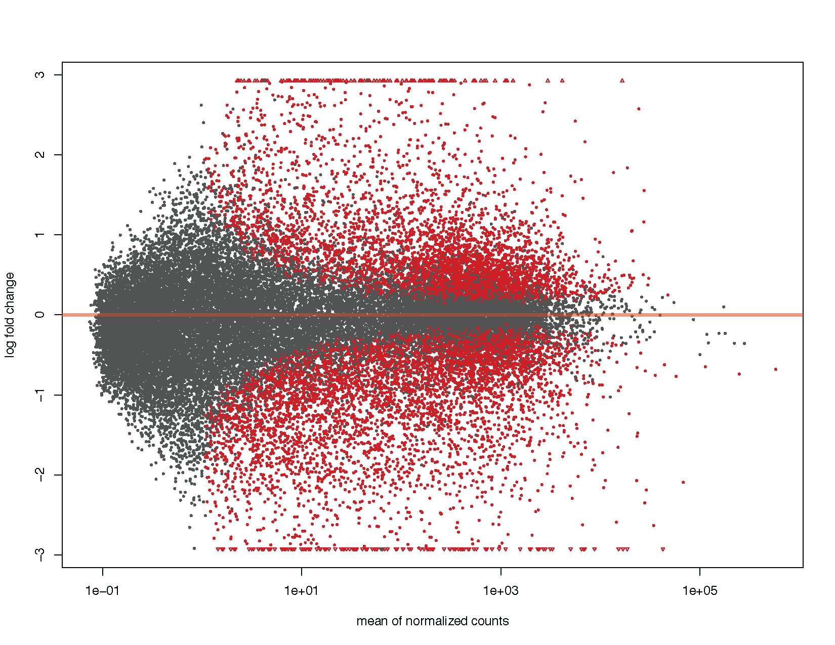
                              # Load libraries                                                # install.packages(c("ggplot2", "scales", "viridis"))                                                library                (                ggplot2                )                                                library                (                scales                )                                                # needed for oob parameter                                                library                (                viridis                )                                                # Coerce to a data frame                                                deseq2ResDF                                                <-                                                equally.data.frame                (                deseq2Results                )                                                # Examine this data frame                                                caput                (                deseq2ResDF                )                                                # Set a boolean column for significance                                                deseq2ResDF                $                significant                                                <-                                                ifelse                (                deseq2ResDF                $                padj                                                <                                                .1                ,                                                "Significant"                ,                                                NA                )                                                # Plot the results similar to DEseq2                                                ggplot                (                deseq2ResDF                ,                                                aes                (                baseMean                ,                                                log2FoldChange                ,                                                colour                =                meaning                ))                                                +                                                geom_point                (                size                =                1                )                                                +                                                scale_y_continuous                (                limits                =                c                (                -iii                ,                                                3                ),                                                oob                =                squish                )                                                +                                                scale_x_log10                ()                                                +                                                geom_hline                (                yintercept                                                =                                                0                ,                                                color                =                "tomato1"                ,                                                size                =                2                )                                                +                                                labs                (                x                =                "hateful of normalized counts"                ,                                                y                =                "log fold alter"                )                                                +                                                scale_colour_manual                (                proper name                =                "q-value"                ,                                                values                =                (                "Significant"                =                "crimson"                ),                                                na.value                =                "grey50"                )                                                +                                                theme_bw                ()                                                # Allow's add some more detail                                                ggplot                (                deseq2ResDF                ,                                                aes                (                baseMean                ,                                                log2FoldChange                ,                                                color                =                padj                ))                                                +                                                geom_point                (                size                =                ane                )                                                +                                                scale_y_continuous                (                limits                =                c                (                -three                ,                                                3                ),                                                oob                =                squish                )                                                +                                                scale_x_log10                ()                                                +                                                geom_hline                (                yintercept                                                =                                                0                ,                                                colour                =                "darkorchid4"                ,                                                size                =                1                ,                                                linetype                =                "longdash"                )                                                +                                                labs                (                10                =                "mean of normalized counts"                ,                                                y                =                "log fold change"                )                                                +                                                scale_colour_viridis                (                management                =                -1                ,                                                trans                =                'sqrt'                )                                                +                                                theme_bw                ()                                                +                                                geom_density_2d                (                colour                =                "blackness"                ,                                                size                =                2                )                                                          

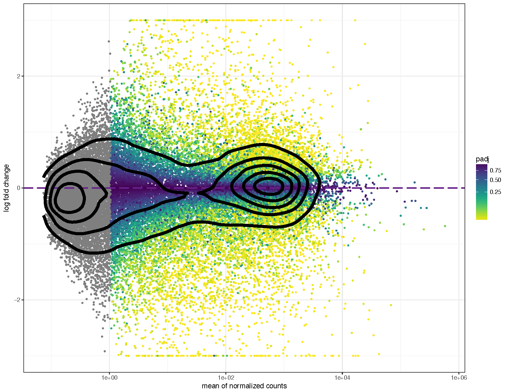
We can see from the to a higher place plots that they are in the feature trumpet shape of MA plots. Further we have overlayed density contours in the second plot and, equally expected, these density contours are centered around a y-intercept of 0. We tin can further run into that equally the average counts increase there is more than ability to telephone call a factor as differentially expressed based on the fold change. You'll besides find that we have quite a few points without an adjusted p-value on the left side of the x-axis. This is occurring because the results() function automatically performs contained filtering using the hateful of normalized counts. This is done to increase the ability to detect an event by not testing those genes which are unlikely to be pregnant based on their high dispersion.

Viewing normalized counts for a single geneID

Frequently it will exist useful to plot the normalized counts for a single gene in lodge to get an idea of what is occurring for that gene across the sample cohort. Fortunately the plotCounts() function from DEseq2 will extract the data we demand for plotting this.

                              # Extract counts for the gene otop2                                                otop2Counts                                                <-                                                plotCounts                (                deseq2Data                ,                                                gene                =                "ENSG00000183034"                ,                                                intgroup                =                c                (                "tissueType"                ,                                                "individualID"                ),                                                returnData                =                TRUE                )                                                # Plot the data using ggplot2                                                colourPallette                                                <-                                                c                (                "#7145cd"                ,                "#bbcfc4"                ,                "#90de4a"                ,                "#cd46c1"                ,                "#77dd8e"                ,                "#592b79"                ,                "#d7c847"                ,                "#6378c9"                ,                "#619a3c"                ,                "#d44473"                ,                "#63cfb6"                ,                "#dd5d36"                ,                "#5db2ce"                ,                "#8d3b28"                ,                "#b1a4cb"                ,                "#af8439"                ,                "#c679c0"                ,                "#4e703f"                ,                "#753148"                ,                "#cac88e"                ,                "#352b48"                ,                "#cd8d88"                ,                "#463d25"                ,                "#556f73"                )                                                ggplot                (                otop2Counts                ,                                                aes                (                x                =                tissueType                ,                                                y                =                count                ,                                                colour                =                individualID                ,                                                group                =                individualID                ))                                                +                                                geom_point                ()                                                +                                                geom_line                ()                                                +                                                theme_bw                ()                                                +                                                theme                (                axis.text.x                =                element_text                (                angle                =                fifteen                ,                                                hjust                =                1                ))                                                +                                                scale_colour_manual                (                values                =                colourPallette                )                                                +                                                guides                (                colour                =                guide_legend                (                ncol                =                iii                ))                                                +                                                ggtitle                (                "OTOP2"                )                                                          

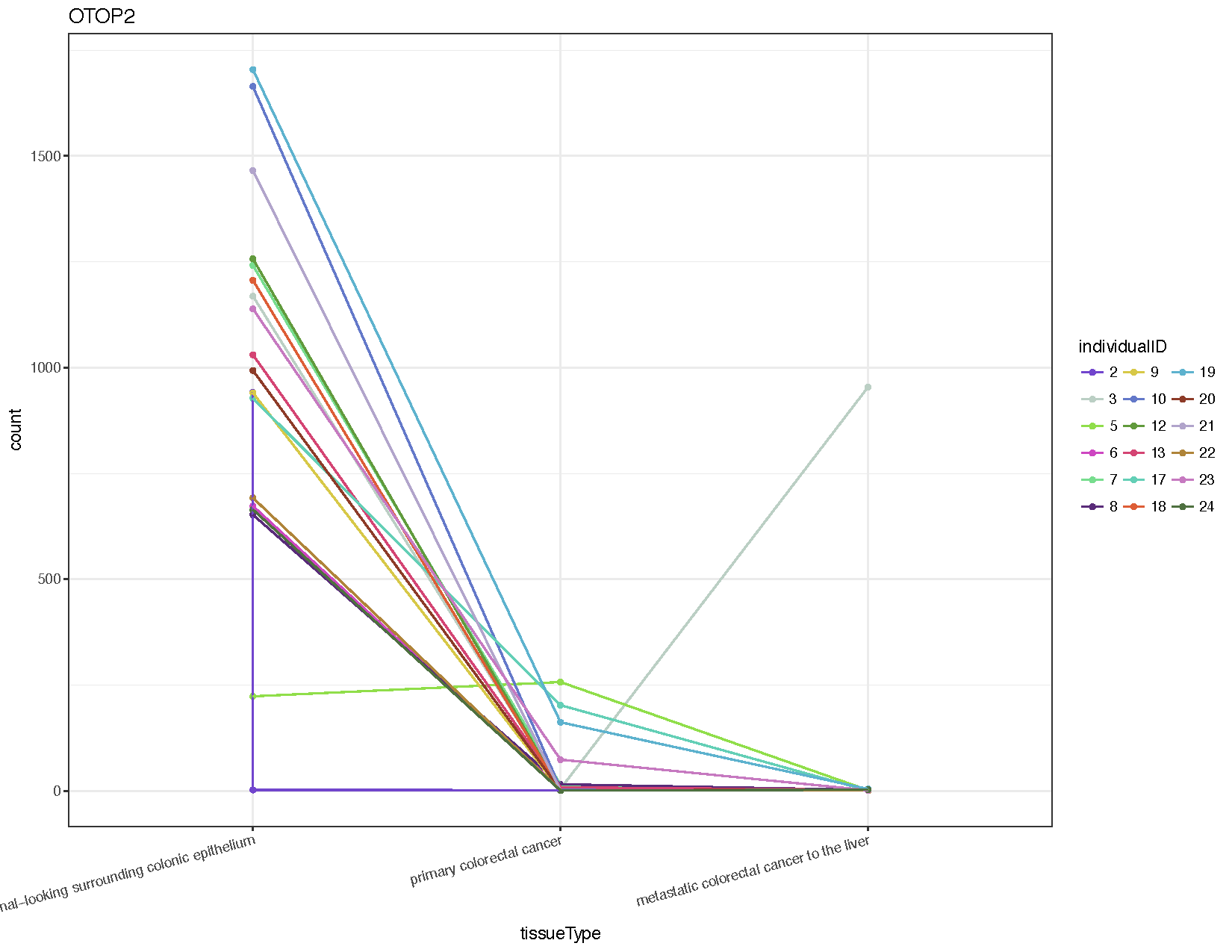
From the resulting plot (meet above) we can see that well-nigh all individuals show down-regulation of this factor in both the principal tumor and metastasis samples compared to the normal. Nosotros've as well introduced a few new ggplot2 concepts, so permit'southward briefly go over them.

  • You will detect that we have specified a group when nosotros initialized our plot. By default ggplot would take assumed the groups were for the discrete variables plotted on the x-axis, and when connecting points with geom_line() this would accept continued all points for each discrete variable instead of connecting by the private id. Try removing the group to get a sense of what happens.
  • We take also altered the legend using guides() to specify the legend to deed on, and guide_legend() to specify that the colour legend should have 3 columns for values instead of just 1.
  • Lastly we accept added a main title with ggtitle(). Yous might accept noticed that individual two looks a little off, specifically based on the plot nosotros created there appears to exist ii normal samples for this individual. Looking at our sample information nosotros tin can observe that this is indeed the case, contrary to the stated experimental design. Looking at the sampleData dataframe nosotros created, we can run across that our suspicions are correct. Often when visualizing data you will catch potential errors that would have otherwise been missed.

Examine the raw data for this gene. Is the p-value significant for this gene? Does this makes sense when nosotros look back at the raw counts for main tumors and normal samples?

                              deseq2ResDF                [                "ENSG00000183034"                ,]                                                rawCounts                [                "ENSG00000183034"                ,]                                                normals                =                row.names                (                sampleData                [                sampleData                [,                "tissueType"                ]                ==                "normal-looking surrounding colonic epithelium"                ,])                                                primaries                =                row.names                (                sampleData                [                sampleData                [,                "tissueType"                ]                ==                "primary colorectal cancer"                ,])                                                rawCounts                [                "ENSG00000183034"                ,                normals                ]                                                rawCounts                [                "ENSG00000183034"                ,                primaries                ]                                                          

Visualizing expression information with a heatmap

It is often informative to plot a heatmap of differentially expressed genes and to perform unsupervised clustering based on the underlying data to decide sub categories within the experiment. In this case we can endeavor to remedy the error nosotros observed in individual 2. Nosotros can use ggplot and ggdendro for this task, but first we must obtain transformed values from the RNAseq counts. The differential expression analysis started from raw counts and normalized using discrete distributions nevertheless when performing clustering we must remove the dependence of the variance on the mean. In other words we must remove the experiment wide trend in the data earlier clustering. In that location are 2 functions within DEseq2 to transform the data in such a manner, the first is to use a regularized logarithm rlog() and the 2d is the variance stablizing transform vst(). There are pros and cons to each method, we will use vst() hither merely because it is much faster. Past default both rlog() and vst() are blind to the sample design formula given to DEseq2 in DESeqDataSetFromMatrix(). However this is not appropriate if one expects large differences in counts, which tin be explained past the differences in the experimental design. In such cases the blind parameter should exist prepare to False.

                              # Transform count data using the variance stablilizing transform                                                deseq2VST                                                <-                                                vst                (                deseq2Data                )                                                # Convert the DESeq transformed object to a data frame                                                deseq2VST                                                <-                                                analysis                (                deseq2VST                )                                                deseq2VST                                                <-                                                as.data.frame                (                deseq2VST                )                                                deseq2VST                $                Gene                                                <-                                                rownames                (                deseq2VST                )                                                head                (                deseq2VST                )                                                # Keep only the significantly differentiated genes where the fold-change was at least 3                                                sigGenes                                                <-                                                rownames                (                deseq2ResDF                [                deseq2ResDF                $                padj                                                <=                                                .05                                                &                                                abs                (                deseq2ResDF                $                log2FoldChange                )                                                >                                                iii                ,])                                                deseq2VST                                                <-                                                deseq2VST                [                deseq2VST                $                Factor                                                %in%                                                sigGenes                ,]                                                # Catechumen the VST counts to long format for ggplot2                                                library                (                reshape2                )                                                # First compare wide vs long version                                                deseq2VST_wide                                                <-                                                deseq2VST                                                deseq2VST_long                                                <-                                                cook                (                deseq2VST                ,                                                id.vars                =                c                (                "Gene"                ))                                                caput                (                deseq2VST_wide                )                                                caput                (                deseq2VST_long                )                                                # Now overwrite our original data frame with the long format                                                deseq2VST                                                <-                                                cook                (                deseq2VST                ,                                                id.vars                =                c                (                "Gene"                ))                                                # Brand a heatmap                                                heatmap                                                <-                                                ggplot                (                deseq2VST                ,                                                aes                (                10                =                variable                ,                                                y                =                Factor                ,                                                fill                =                value                ))                                                +                                                geom_raster                ()                                                +                                                scale_fill_viridis                (                trans                =                "sqrt"                )                                                +                                                theme                (                axis.text.ten                =                element_text                (                angle                =                65                ,                                                hjust                =                ane                ),                                                axis.text.y                =                element_blank                (),                                                axis.ticks.y                =                element_blank                ())                                                heatmap                                                          

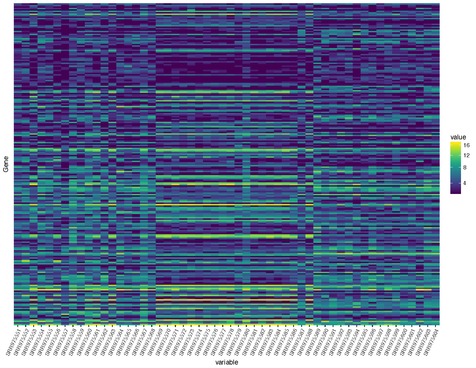
Allow's briefly talk most the steps we took to obtain the heatmap we plotted above.

  • First we took our DESeq2DataSet object we obtained from the command DESeq() and transformed the values using the variance stabilizing tranform algorithm from the vst() function.
  • We then extracted these transformed values with the assay() function and converted the resulting object to a data frame with a column for gene id's.
  • We adjacent used the differential expression results we had previously obtained to filter our transformed matrix to only those genes which were significantly differentially expressed (q-value <= .05) and with a log2 fold change greater than 3.
  • Up to this signal our transformed values have been in "wide" format, yet ggplot2 required long format. We achieve this with melt() function from the reshape2 package.
  • Finally we use ggplot2 and the geom_raster() function to create a heatmap using the colour scheme available from the viridis parcel.

Clustering

At present that nosotros have a heatmap let's start clustering using the functions available with base R.

  • The commencement step is to convert our transformed values back to wide format using dcast() with row names and columns names as genes and samples respectively.
  • Next we can compute a distance matrix using dist() which will compute the distance based on the rows of our data frame. This will give u.s. the distance matrix based on our genes, only we also want a altitude matrix based on the samples, for this we simply have to transpose our matrix before calling dist() with the part t().
  • From in that location nosotros can perform hierarchical clustering with the hclust() function.
  • We and so install the ggdendro package to construct a dendrogram as described in their vignette.
  • Finally we re-create the heatmap to match the dendrogram using the cistron() part to re-order how samples are plotted.
  • Because ggplot plots use grid graphics underneath we tin can use the gridExtra package to combine both plots into i with the function grid.arrange().
                              # Convert the significant genes back to a matrix for clustering                                                deseq2VSTMatrix                                                <-                                                dcast                (                deseq2VST                ,                                                Factor                                                ~                                                variable                )                                                rownames                (                deseq2VSTMatrix                )                                                <-                                                deseq2VSTMatrix                $                Gene                                                deseq2VSTMatrix                $                Gene                                                <-                                                NULL                                                # Compute a distance calculation on both dimensions of the matrix                                                distanceGene                                                <-                                                dist                (                deseq2VSTMatrix                )                                                distanceSample                                                <-                                                dist                (                t                (                deseq2VSTMatrix                ))                                                # Cluster based on the distance calculations                                                clusterGene                                                <-                                                hclust                (                distanceGene                ,                                                method                =                "average"                )                                                clusterSample                                                <-                                                hclust                (                distanceSample                ,                                                method                =                "average"                )                                                # Construct a dendogram for samples                                                install.packages                (                "ggdendro"                )                                                library                (                ggdendro                )                                                sampleModel                                                <-                                                as.dendrogram                (                clusterSample                )                                                sampleDendrogramData                                                <-                                                segment                (                dendro_data                (                sampleModel                ,                                                type                                                =                                                "rectangle"                ))                                                sampleDendrogram                                                <-                                                ggplot                (                sampleDendrogramData                )                                                +                                                geom_segment                (                aes                (                x                                                =                                                x                ,                                                y                                                =                                                y                ,                                                xend                                                =                                                xend                ,                                                yend                                                =                                                yend                ))                                                +                                                theme_dendro                ()                                                # Re-gene samples for ggplot2                                                deseq2VST                $                variable                                                <-                                                gene                (                deseq2VST                $                variable                ,                                                levels                =                clusterSample                $                labels                [                clusterSample                $                order                ])                                                # Construct the heatmap. notation that at this point we have only clustered the samples NOT the genes                                                heatmap                                                <-                                                ggplot                (                deseq2VST                ,                                                aes                (                x                =                variable                ,                                                y                =                Gene                ,                                                fill                =                value                ))                                                +                                                geom_raster                ()                                                +                                                scale_fill_viridis                (                trans                =                "sqrt"                )                                                +                                                theme                (                axis.text.10                =                element_text                (                angle                =                65                ,                                                hjust                =                one                ),                                                centrality.text.y                =                element_blank                (),                                                axis.ticks.y                =                element_blank                ())                                                heatmap                                                # Combine the dendrogram and the heatmap                                                install.packages                (                "gridExtra"                )                                                library                (                gridExtra                )                                                grid.arrange                (                sampleDendrogram                ,                                                heatmap                ,                                                ncol                =                1                ,                                                heights                =                c                (                1                ,                5                ))                                                          

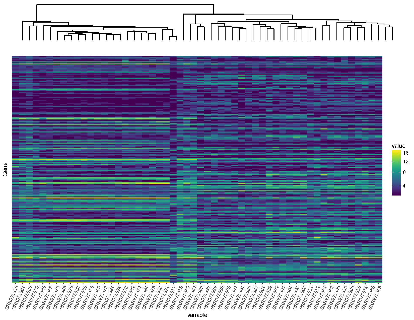
Our graph is looking pretty adept, only you'll observe that the dendrogram plot doesn't line up well with the heatmap plot. This is because the plot widths from our ii plots don't quite match upwardly. This can occur for a variety of reasons. In this example it is because we have a legend in one plot merely not in the other. Fortunately this sort of problem is generally easy to fix.

                              # Load in libraries necessary for modifying plots                                                #install.packages("gtable")                                                library                (                gtable                )                                                library                (                grid                )                                                # Modify the ggplot objects                                                sampleDendrogram_1                                                <-                                                sampleDendrogram                                                +                                                scale_x_continuous                (                expand                =                c                (                .0085                ,                                                .0085                ))                                                +                                                scale_y_continuous                (                expand                =                c                (                0                ,                                                0                ))                                                heatmap_1                                                <-                                                heatmap                                                +                                                scale_x_discrete                (                expand                =                c                (                0                ,                                                0                ))                                                +                                                scale_y_discrete                (                expand                =                c                (                0                ,                                                0                ))                                                # Convert both grid based objects to grobs                                                sampleDendrogramGrob                                                <-                                                ggplotGrob                (                sampleDendrogram_1                )                                                heatmapGrob                                                <-                                                ggplotGrob                (                heatmap_1                )                                                # Check the widths of each grob                                                sampleDendrogramGrob                $                widths                                                heatmapGrob                $                widths                                                # Add together in the missing columns                                                sampleDendrogramGrob                                                <-                                                gtable_add_cols                (                sampleDendrogramGrob                ,                                                heatmapGrob                $                widths                [                vii                ],                                                6                )                                                sampleDendrogramGrob                                                <-                                                gtable_add_cols                (                sampleDendrogramGrob                ,                                                heatmapGrob                $                widths                [                8                ],                                                seven                )                                                # Make sure every width between the 2 grobs is the same                                                maxWidth                                                <-                                                unit.pmax                (                sampleDendrogramGrob                $                widths                ,                                                heatmapGrob                $                widths                )                                                sampleDendrogramGrob                $                widths                                                <-                                                every bit.listing                (                maxWidth                )                                                heatmapGrob                $                widths                                                <-                                                as.list                (                maxWidth                )                                                # Accommodate the grobs into a plot                                                finalGrob                                                <-                                                arrangeGrob                (                sampleDendrogramGrob                ,                                                heatmapGrob                ,                                                ncol                =                ane                ,                                                heights                =                c                (                2                ,                5                ))                                                # Depict the plot                                                grid.draw                (                finalGrob                )                                                          

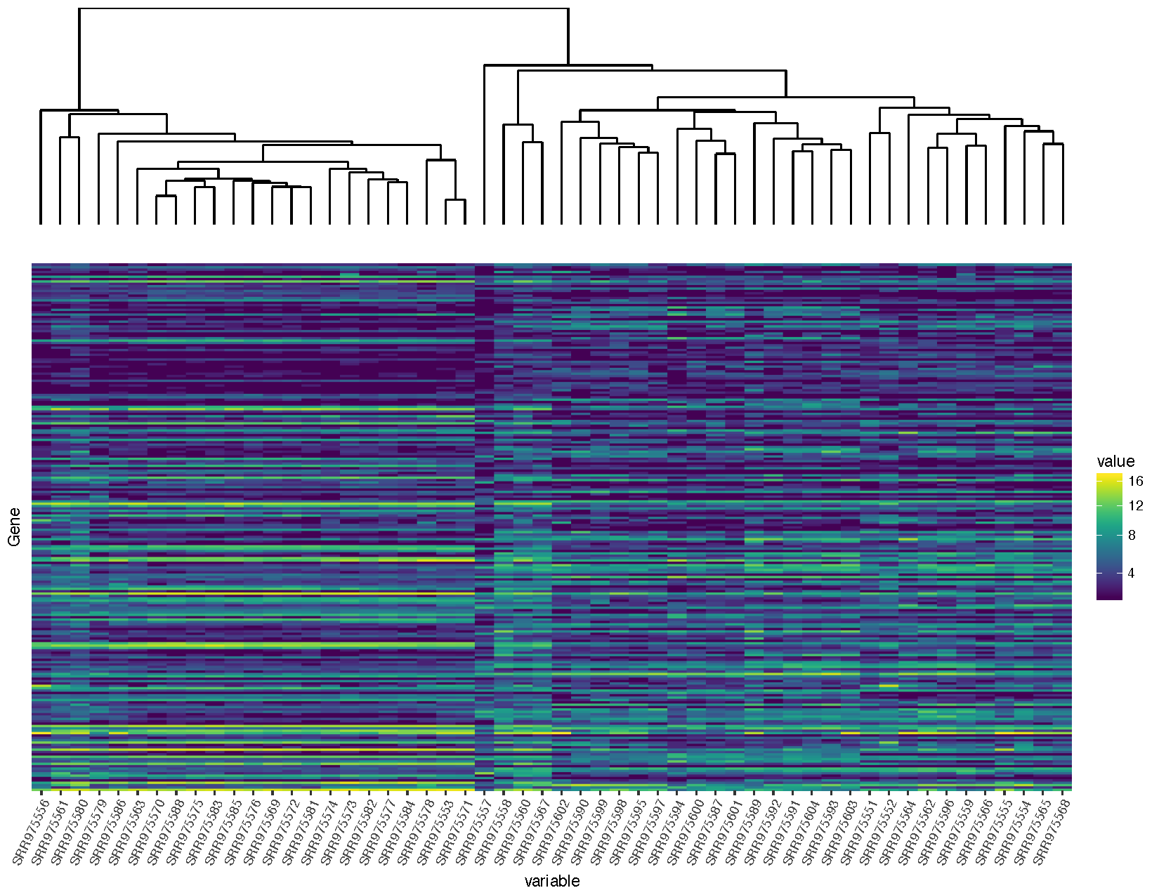
You will notice that we are loading in a few additional packages to help solve this problem. All plots within ggplot are at the everyman level graphical objects (grobs) from the filigree parcel. The gtable allows u.s. to view and manipulate these grobs as tables making them easier to work with.

  • The first pace later on loading these packages is to alter the x-axis scales in our plots. Past default ggplot adds a padding inside all plots so data is not plotted on the border of the plot. Nosotros tin can control this padding with the expand parameter inside ggplot'south scale layers. To go things just right you will demand to alter these parameters and so data within the plots line upwards, estimate alterations are provided to a higher place so let's move on the the side by side step.
  • Nosotros need to make certain the chief panels in both plots line up exactly, in lodge to practise this we must first convert these plots to tabular array grobs to make them easier to manipulate, this is accomplished with the ggplotGrob() role.
  • Now that these are grobs we compare the widths of each grob, yous might discover that two widths seem to be missing from the the dendrogram plot. These 2 widths correspond to the legend in the heatmap, we use the gtable_add_cols() function to insert in the widths for these two elements from the heatmap grob into the dendrogram grob.
  • The next step is to then find the maximum widths for each grob object using unit.pmax() and to overwrite each grobs width with these maximum widths.
  • Finally we accommodate the grobs on the page we are plotting to using arrangeGrob() and draw the final plot with grid.draw().

Now that we've completed that allow's add a plot between the dendrogram and the heatmap showing the tissue blazon to try and discern which normal sample in individual two should be the metastasis sample equally per the experimental design described.

                              # Re-order the sample data to friction match the clustering we did                                                sampleData_v2                $                Run                                                <-                                                factor                (                sampleData_v2                $                Run                ,                                                levels                =                clusterSample                $                labels                [                clusterSample                $                gild                ])                                                # Construct a plot to show the clinical data                                                colours                                                <-                                                c                (                "#743B8B"                ,                                                "#8B743B"                ,                                                "#8B3B52"                )                                                sampleClinical                                                <-                                                ggplot                (                sampleData_v2                ,                                                aes                (                x                =                Run                ,                                                y                =                1                ,                                                fill up                =                Sample.Feature.biopsy.site.                ))                                                +                                                geom_tile                ()                                                +                                                scale_x_discrete                (                aggrandize                =                c                (                0                ,                                                0                ))                                                +                                                scale_y_discrete                (                expand                =                c                (                0                ,                                                0                ))                                                +                                                scale_fill_manual                (                name                =                "Tissue"                ,                                                values                =                colours                )                                                +                                                theme_void                ()                                                # Convert the clinical plot to a grob                                                sampleClinicalGrob                                                <-                                                ggplotGrob                (                sampleClinical                )                                                # Make certain every width between all grobs is the aforementioned                                                maxWidth                                                <-                                                unit.pmax                (                sampleDendrogramGrob                $                widths                ,                                                heatmapGrob                $                widths                ,                                                sampleClinicalGrob                $                widths                )                                                sampleDendrogramGrob                $                widths                                                <-                                                as.list                (                maxWidth                )                                                heatmapGrob                $                widths                                                <-                                                as.list                (                maxWidth                )                                                sampleClinicalGrob                $                widths                                                <-                                                as.list                (                maxWidth                )                                                # Arrange and output the final plot                                                finalGrob                                                <-                                                arrangeGrob                (                sampleDendrogramGrob                ,                                                sampleClinicalGrob                ,                                                heatmapGrob                ,                                                ncol                =                i                ,                                                heights                =                c                (                2                ,                ane                ,                v                ))                                                grid.draw                (                finalGrob                )                                                          

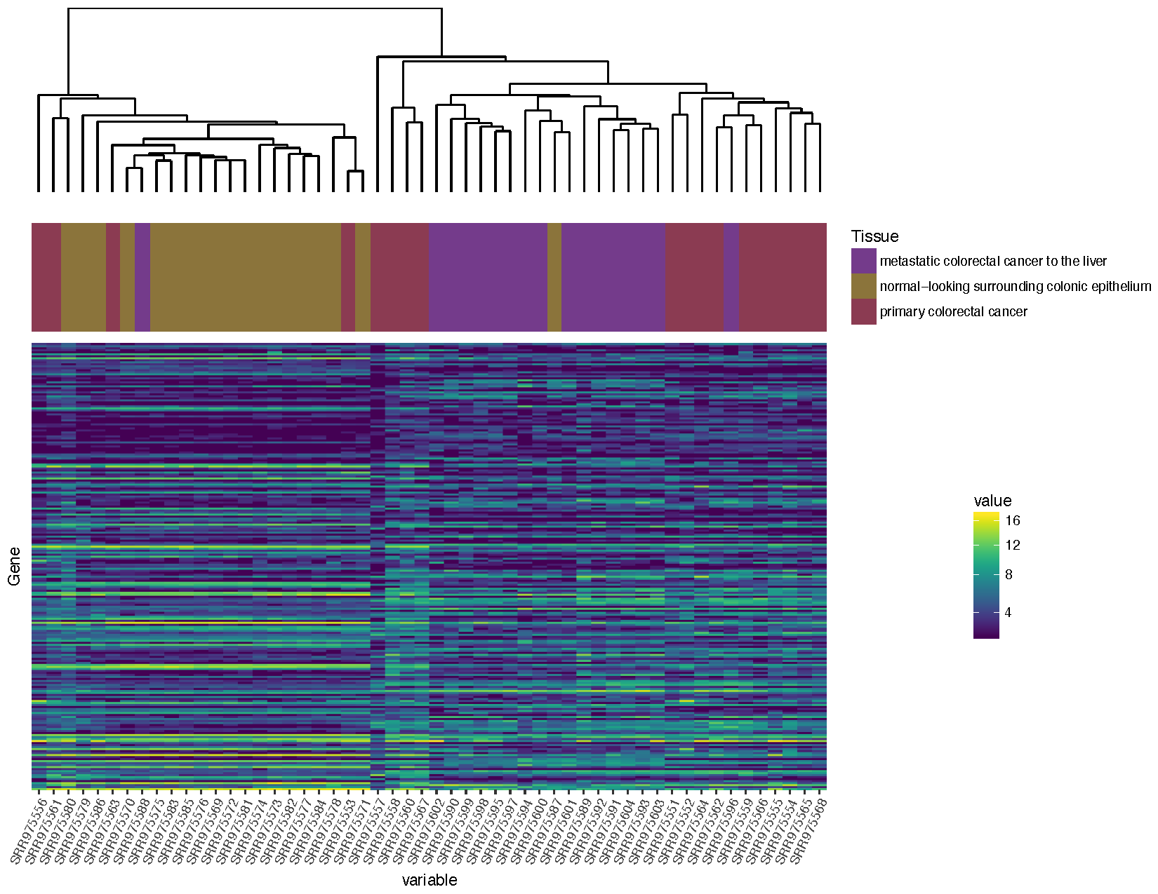
Based on the plot yous produced above, which normal sample for private 2 is likely the metastasis sample

Based on the clustering, sample SRR975587

Exercises

In the tutorial in a higher place we have completed the steps necessary to produce a dendrogram for samples, we could also do this for genes. Endeavour to reproduce the plot below, if y'all get stuck you lot'll find an rscript that below which will produce the right answer! Your steps should look something like this:

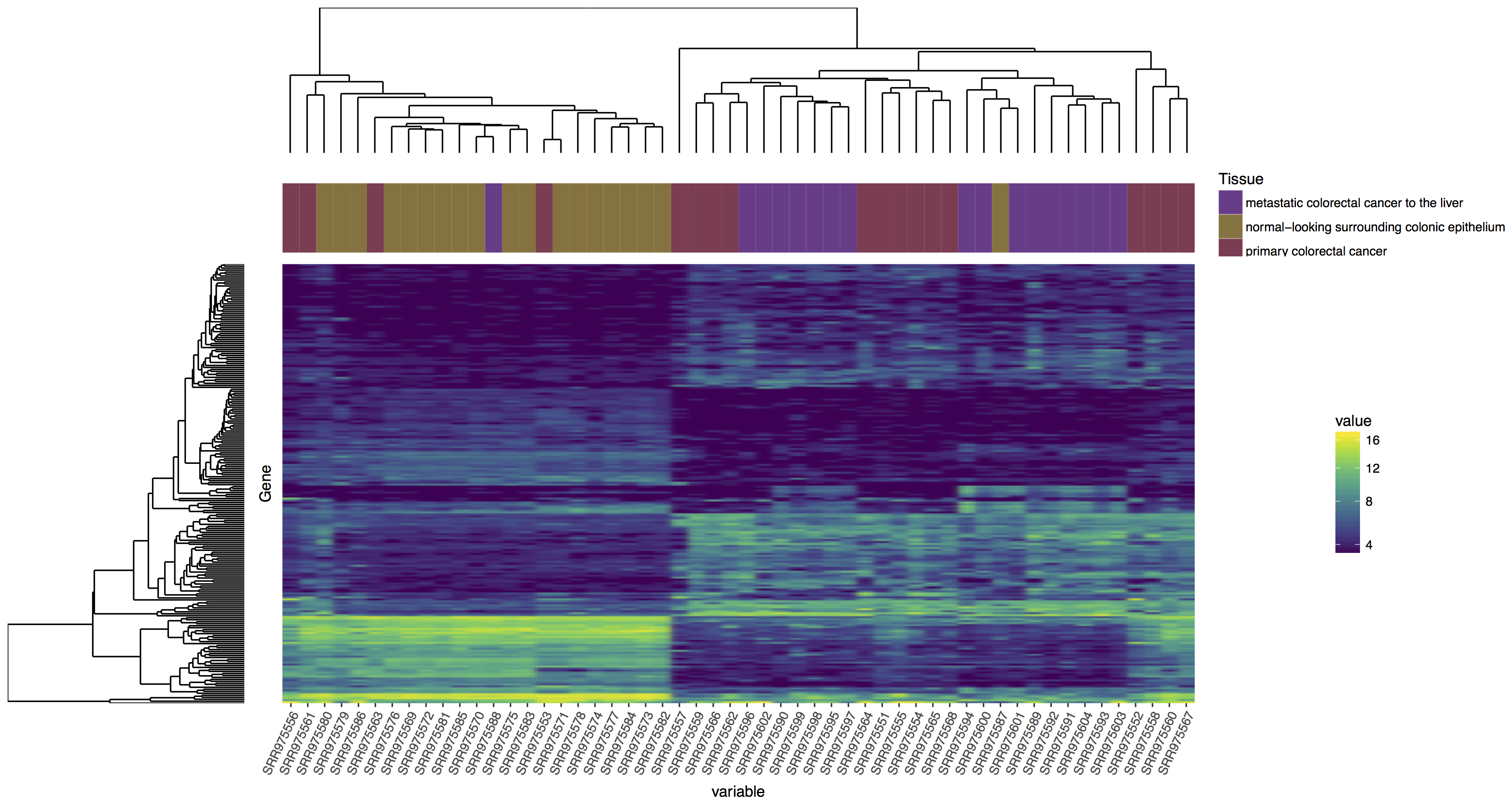
  1. Create a dendrogram for genes
    1. use coord_flip() and scale_y_reverse()
  2. re-accommodate the factor cells on the y-axis to match the gene dendrogram
  3. convert the dendrogram and heatmaps to grobs
  4. marshal the cistron dendrogram heights to match the heatmap (annotation: you don't need to worry nearly the legend in this example)
    1. you'll likewise need to repeat the tutorial steps for aligning the sample dendrogram since we take a new heatmap, consider this step 4B.
    2. annotation that yous tin can use unit.pmax to help you make up one's mind the max elevation and width of your grobs
  5. create a bare panel you can apply this: blankPanel<-grid.rect(gp=gpar(col="white"))
  6. use the gridExtra package to position the panels and plot the result.

Reproduce the plot above, follow the steps outlined.

This Rscript file contains the correct answer.

How To Filter Genes With Zero Reads In Count File Deseq2,

Source: https://genviz.org/module-04-expression/0004/02/01/DifferentialExpression/

Posted by: boazyourne1946.blogspot.com

0 Response to "How To Filter Genes With Zero Reads In Count File Deseq2"

Post a Comment

Iklan Atas Artikel

Iklan Tengah Artikel 1

Iklan Tengah Artikel 2

Iklan Bawah Artikel